The AI That Babysits Qubits

Under every “quantum computers don't work yet” headline sits a pattern-recognition problem, and an AI now reads that pattern better than the rules people wrote for it. Pick a depth below. The depth you pick is part of the link, so a page you share opens at the same depth for whoever you send it to.

You'll be able to say why a quantum computer needs constant error correction, and what an AI decoder adds.

One analogy, no equations, about two minutes. The Working tier builds the machinery and Formal carries the derivation.

A quantum computer is a choir in which every singer slowly drifts off key, and glancing at any one of them to check makes that singer forget the song. (Singer = qubit, the machine's basic unit of information. Off key = the small error every qubit collects simply by existing. Those are the only two terms you need.)

Read that twice, because it is the knot every quantum engineer is trying to untie: you cannot fix what you are not allowed to look at.

Error correction hires a conductor who never listens to a soloist. The only question they put, to one neighbouring pair at a time, is do you two match? Since nobody is heard alone, nobody forgets the song, and two clashes side by side still point straight at the singer who drifted.

For thirty years the conductor's rulebook was written by hand. In 2024 Google DeepMind trained an AI, AlphaQubit, to write its own, by listening to one real choir's recordings until it learned that choir's bad habits. It makes about 30% fewer wrong calls than the hand-written rulebooks fast enough to run on a live machine, and about 6% fewer than the slowest and most careful one. It is still too slow to conduct a live performance, and making it fast enough is the race everyone is now running.

The mechanism, one worked number, and the picture you should have in your head. No derivations; those are in Formal.

The mechanism

Physical qubits fail constantly, roughly 1 error per 1,000 operations on good hardware. The fix is not a better qubit; it is redundancy with a twist. You encode one logical qubit across many physical ones in a surface code, then never measure the data at all.

Instead, extra measurement qubits sitting between the data qubits run parity checks, the syndrome measurements. Each one asks only whether its neighbours agree, never what they are. Everything hangs on that distinction: a parity check extracts the fact that something flipped without extracting the value that would collapse the superposition. A decoder then infers the most likely error pattern from the history of those checks, the way a doctor diagnoses from symptoms rather than by opening the patient.

The picture to hold in your head

Draw a checkerboard. Every corner is a data qubit, holding part of your one logical qubit. Every square is a measurement qubit that watches the four corners touching it and reports a single bit: even or odd. The squares alternate between two flavours (one watches for bit flips, the other for phase flips) because a qubit can fail in two independent ways and you need to catch both.

Run every square once and you get a snapshot: mostly zeros, with a few squares lit up. A single flipped data qubit lights the squares around it. A chain of flips lights only the two squares at its ends; everything in the middle cancels. So the decoder never sees the error, it sees a scattering of endpoints and has to guess the cheapest set of chains that would produce exactly those endpoints. That is why decoding is a matching problem, and why a 1965 graph algorithm ended up inside a quantum computer.

The number that explains the whole overhead

Here is the one calculation worth doing by hand, because it explains every "1,000 qubits to make 1" headline you have read.

A useful algorithm runs on the order of a billion logical operations. For fewer than one expected failure across the whole run, you need a logical error rate below about 10⁻⁹. You are starting from a physical error rate of 10⁻³. So the code has to buy you six orders of magnitude.

It buys them in steps. Each increase of the code distance d by two multiplies the suppression by a factor Λ. Google measured Λ = 2.14 on Willow, fitted across its whole d = 3, 5, 7 series. So a factor of 1,000 costs about nine of those steps: 2.14⁹ ≈ 941.

Nine steps takes you from d = 5 to d = 23. A rotated surface-code patch at distance d costs 2d² − 1 physical qubits, so that one logical qubit now occupies 1,057 physical qubits, and you have bought roughly 1,000×, not the full million. That is the exchange rate. It is also why Λ is the single most important number in the field: it is the interest rate on every qubit you will ever build.

Where the AI walked in

The classic decoder, minimum-weight perfect matching, assumes errors are independent and simple. Real hardware is not: errors correlate across neighbours, qubits leak out of the computational space entirely, and the noise drifts between calibrations. Matching cannot express any of that, because its model has no vocabulary for it.

AlphaQubit is a recurrent transformer trained first on hundreds of millions of simulated samples, then fine-tuned on thousands of samples from the real chip, so it learns the actual noise rather than the idealised model, and it reads the analog "soft" readout signal instead of a hard 0/1. Result: about 30% fewer logical errors than correlated matching, the fast class you can run live.

The catch is the return arrow in the diagram above. The decoder has to finish inside the cycle, or the backlog grows forever, so an accurate decoder that is too slow does not count. That, not accuracy, is the open engineering problem.

Formalism, one derivation carried through, primary sources, and the problems still open. Assumes stabilizer formalism. The Working tier carries the same content without the algebra. Independently verified 2026-07-13.

Rotated surface code with code distance d: d² data qubits, d²−1 syndrome qubits, so a patch costs 2d²−1 physical qubits. Stabilizers are weight-4 X/Z plaquette operators in the bulk (weight-2 on boundaries), measured each cycle. Decoding is inference over the syndrome volume: given syndrome history σ, find the most probable logical equivalence class of errors, not the most probable error, which is a different and worse objective.

Where the exponent comes from

The scaling law quoted everywhere is worth deriving once, because the exponent is where the recurring off-by-one in this field lives.

A distance-d code corrects any error of weight t = ⌊(d−1)/2⌋. So the lowest-order event the decoder cannot fix requires t+1 = ⌊(d+1)/2⌋ physical faults. Below threshold each independent fault carries probability ∝ p, and the number of weight-(t+1) fault patterns is a binomial prefactor in the patch size. Summing the lowest-order term:

with A and p_th absorbing the combinatorics and the decoder's quality. Two consequences follow immediately, and both are routinely stated wrong:

• Raising an odd d by one buys nothing. ⌊(d+1)/2⌋ is unchanged from d = 23 to d = 24. This is why the literature always steps d → d+2, and why "distance" and "step" must never be used interchangeably in the same paragraph.
• Λ is defined per two-distance step. Λ ≡ p_L(d) / p_L(d+2). Google's measured Λ = 2.14 ± 0.02 on Willow comes from a linear regression of ln(ε_d) against d across its whole d = 3, 5, 7 series (Nature 638, 920 (2025)) — not from any single step: the lone d = 5 → 7 ratio is ≈ 2.12. It is not a per-unit-distance figure.

Working the exchange rate the other way: buying 10³ suppression at Λ = 2.14 needs log(10³)/log(2.14) ≈ 9.08 steps, so nine steps gives 2.14⁹ ≈ 941×, taking d = 5 → 23 and one logical qubit to 2(23²)−1 = 1,057 physical qubits. The million-fold suppression a billion-operation algorithm needs costs roughly double that distance again.

Note what the ratio construction buys you: expressing everything relative to d = 3 cancels the unknown prefactor A exactly, so the suppression curve is a parameter-free prediction rather than a fit. Real devices depart from it near threshold, where the lowest-order truncation stops being enough.

Decoders

MWPM solves the inference on a decoder graph with edge weights drawn from an assumed independent-Pauli plus phenomenological noise model: provably good under that model, degraded under correlated noise, leakage, cross-talk and non-Markovian drift. The failure is structural rather than computational: the model has no term for the thing that is happening.

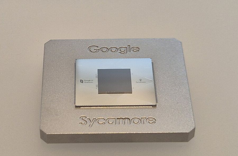
AlphaQubit: recurrent transformer over per-round syndrome inputs, including analog "soft" readout rather than binarized measurements, which hands it more information to work with, on top of being a bigger model. Pretrained on hundreds of millions of simulated samples, fine-tuned on thousands of experimental samples from a Sycamore processor. Reported ~6% fewer logical errors than tensor-network decoders (near-optimal, far too slow for real time) and ~30% fewer than correlated matching. The real-device data is d = 3 and d = 5; the d = 11 result is simulation only, a distinction frequently lost in secondary coverage, and one we got wrong here once — caught in editing, before the corrections log started counting.

Below threshold, a decoder that effectively raises p_th or sharpens the exponent compounds through every future distance increase. Decoder quality is hardware you do not have to build, which is the entire economic argument for this site's thesis.

What is still open

Stated as problems rather than as a roadmap, because for most of them the truthful answer is that nobody knows yet.

1. Real-time decoding at scale. "NN decoders are too slow for the ~1 μs cycle" is no longer simply true: an FPGA neural decoder hit 550 ns system latency (124 ns inference) inside a 1.25 μs cycle on superconducting hardware (arXiv:2605.04892, May 2026). But that is small d. Latency and bandwidth both grow with patch size while the cycle budget does not, and no published learned decoder runs in real time at the distances fault tolerance requires.
2. Whether the learned margin survives scale. Every reported advantage for learned decoders is measured at small distance. There is no result showing the ~30% margin holds at d = 25 or beyond, and there is no theory saying it must.
3. Leakage and non-Markovian noise. Both sit outside the Pauli model that the threshold theorem's guarantees are stated in. Leakage-reduction units exist and cost cycles; the accounting for how much they cost at scale is not settled.
4. Magic states dominate the real bill. Clifford operations are the easy half, essentially free under the code. Non-Clifford gates need distilled magic states, and T-count, not qubit count, sets the wall-clock time for any real algorithm. Resource estimates move by orders of magnitude when distillation architectures change, which is exactly what happened to the Bitcoin numbers between 2022 and 2026.
5. Threshold versus pseudo-threshold. The single number "p_th ≈ 1%" is model-, decoder- and geometry-dependent. Quoting it without those three qualifiers is the most common way this field's own literature is misread.

Primary sources